42 how do you add data labels to a chart in excel
peltiertech.com › add-horizontal-line-to-excel-chartAdd a Horizontal Line to an Excel Chart - Peltier Tech Sep 11, 2018 · Paste Special. If you don’t use Paste Special often, it might be hard to find. If you copy a range and use the right click menu on a chart, the only option is a regular Paste, and Excel doesn’t always correctly guess how it should paste the data. How do you change chart labels to percentages? - Evanewyork.net To add data labels in Excel 2013 or Excel 2016, follow these steps: Activate the chart by clicking on it, if necessary. Make sure the Design tab of the ribbon is displayed. Click the Add Chart Element drop-down list. Select the Data Labels tool. Select the position that best fits where you want your labels to appear. How do you convert data ...
How to Add Axis Titles in a Microsoft Excel Chart - How-To Geek Select your chart and then head to the Chart Design tab that displays. Click the Add Chart Element drop-down arrow and move your cursor to Axis Titles. In the pop-out menu, select "Primary Horizontal," "Primary Vertical," or both. If you're using Excel on Windows, you can also use the Chart Elements icon on the right of the chart.

How do you add data labels to a chart in excel
› documents › excelHow to add data labels from different column in an Excel chart? This method will introduce a solution to add all data labels from a different column in an Excel chart at the same time. Please do as follows: 1. Right click the data series in the chart, and select Add Data Labels > Add Data Labels from the context menu to add data labels. 2. Data Labels in Excel Pivot Chart (Detailed Analysis) Next open Format Data Labels by pressing the More options in the Data Labels. Then on the side panel, click on the Value From Cells. Next, in the dialog box, Select D5:D11, and click OK. Right after clicking OK, you will notice that there are percentage signs showing on top of the columns. 4. Changing Appearance of Pivot Chart Labels Excel - adding new data points to an existing chart I am trying to add data points to an existing chart. The new data has been added to the table in the related spreadsheet. When I right-click on one of the three series shown in my chart and then choosing "select data" the Select Data Source window which appears states that "the data range is too complex to be displayed".
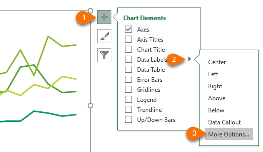
How do you add data labels to a chart in excel. How to Print Labels from Excel - Lifewire To label legends in Excel, select a blank area of the chart. In the upper-right, select the Plus ( +) > check the Legend checkbox. Then, select the cell containing the legend and enter a new name. How do I label a series in Excel? To label a series in Excel, right-click the chart with data series > Select Data. › how-to-create-excel-pie-chartsHow to Make a Pie Chart in Excel & Add Rich Data Labels to ... Sep 08, 2022 · In this article, we are going to see a detailed description of how to make a pie chart in excel. One can easily create a pie chart and add rich data labels, to one’s pie chart in Excel. So, let’s see how to effectively use a pie chart and add rich data labels to your chart, in order to present data, using a simple tennis related example. Adding Data Labels to Your Chart (Microsoft Excel) - ExcelTips (ribbon) To add data labels in Excel 2013 or later versions, follow these steps: Activate the chart by clicking on it, if necessary. Make sure the Design tab of the ribbon is displayed. (This will appear when the chart is selected.) Click the Add Chart Element drop-down list. Select the Data Labels tool. How to add data labels in excel to graph or chart (Step-by-Step) Add data labels to a chart. 1. Select a data series or a graph. After picking the series, click the data point you want to label. 2. Click Add Chart Element Chart Elements button > Data Labels in the upper right corner, close to the chart. 3. Click the arrow and select an option to modify the location. 4.
How to Add Total Values to Stacked Bar Chart in Excel Step 4: Add Total Values. Next, right click on the yellow line and click Add Data Labels. Next, double click on any of the labels. In the new panel that appears, check the button next to Above for the Label Position: Next, double click on the yellow line in the chart. In the new panel that appears, check the button next to No line: A Step-by-Step Guide on How to Make a Graph in Excel - Simplilearn.com Follow the steps mentioned below to create a simple histogram. Select the data from the sheet on which you want to make a histogram. Click on the Insert Tab, you will find the Insert Statistic Chart option in the Charts group. A drop down will appear from where you can select the desired histogram chart. How to Add Leader Lines in Excel? - GeeksforGeeks Step 1: Select a range of cells for which you want to make a line chart. Step 2: Go to Insert Tab and select Recommended Charts. A dialogue box name Insert Chart appears. Step 3: Click on All Charts and select Line. Click Ok. Step 4: A line chart is embedded in the worksheet. Step 5: Go to Chart Design Tab and select Add Chart Element . How to add a line in Excel graph: average line, benchmark, etc. In the Select Data Source dialog box, click the Add button in the Legend Entries (Series) In the Edit Series dialog window, do the following: In the Series name box, type the desired name, say "Target line". Click in the Series value box and select your target values without the column header. Click OK twice to close both dialog boxes.
How To Add an Equation To a Graph in Excel (Step-by-Step Guide) Here are the steps to add an equation to a graph in Microsoft Excel: 1. Enter data into Excel. The first step is to open the application on your computer or by accessing it through your web browser. Once on the homepage, navigate to the worksheet and begin entering your data to create a table. For a typical linear graph, you can create two ... How to Apply a Filter to a Chart in Microsoft Excel - How-To Geek Select the chart and you'll see buttons display to the right. Click the Chart Filters button (funnel icon). When the filter box opens, select the Values tab at the top. You can then expand and filter by Series, Categories, or both. Simply check the options you want to view on the chart, then click "Apply." How to Edit Pie Chart in Excel (All Possible Modifications) Just like the chart title, you can also change the position of data labels in a pie chart. Follow the steps below to do this. 👇 Steps: Firstly, click on the chart area. Following, click on the Chart Elements icon. Subsequently, click on the rightward arrow situated on the right side of the Data Labels option. How to Add Data Labels to Scatter Plot in Excel (2 Easy Ways) - ExcelDemy Then, go to the Insert tab. After that, select Insert Scatter (X, Y) or Bubble Chart > Scatter. At this moment, we can see the Scatter Plot visualizing our data table. Secondly, go to the Chart Design tab. Now, select Add Chart Element from the ribbon. From the drop-down list, select Data Labels.
How to Add Data Labels to your Excel Chart in Excel 2013
How to Add Axis Labels in Microsoft Excel - Appuals.com Click on the Chart Elements button (represented by a green + sign) next to the upper-right corner of the selected chart. Enable Axis Titles by checking the checkbox located directly beside the Axis Titles option. Once you do so, Excel will add labels for the primary horizontal and primary vertical axes to the chart.

How to Change Excel Chart Data Labels to Custom Values?
How to Add Secondary Axis in Excel (3 Useful Methods) - ExcelDemy 2) Now go to Insert tab => click on the Recommended Charts command in the Charts window or click on the little arrow icon on the bottom right corner of the window. 3) This will open the Insert Chart dialog box. In the Insert Chart dialog box, choose the All Charts tab. Then choose the Combo option from the left menu.

How to add or move data labels in Excel chart?
› excel › how-to-add-total-dataHow to Add Total Data Labels to the Excel Stacked Bar Chart Apr 03, 2013 · Step 4: Right click your new line chart and select “Add Data Labels” Step 5: Right click your new data labels and format them so that their label position is “Above”; also make the labels bold and increase the font size. Step 6: Right click the line, select “Format Data Series”; in the Line Color menu, select “No line” Step 7 ...

Add Total Values for Stacked Column and Stacked Bar Charts in ...
Use defined names to automatically update a chart range - Office Select cells A1:B4. On the Insert tab, click a chart, and then click a chart type.. Click the Design tab, click the Select Data in the Data group.. Under Legend Entries (Series), click Edit.. In the Series values box, type =Sheet1!Sales, and then click OK.. Under Horizontal (Category) Axis Labels, click Edit.. In the Axis label range box, type =Sheet1!Date, and then click OK.

How to Use Cell Values for Excel Chart Labels
How to make a quadrant chart using Excel | Basic Excel Tutorial Add values to the chart. 1. Right-click on the empty chart area and choose 'Select Data.' 2. A new window, "Select Data Source," will be displayed. Under the 'Legend Entries (Series)' field, click the "Add" button. 3. The 'Edit Series' menu will be displayed.

Adding rich data labels to charts in Excel 2013 | Microsoft ...
How to add trendline in Excel chart - Ablebits.com To add a trendline in Excel 2010, you follow a different route: On a chart, click the data series for which you want to draw a trendline. Under Chart Tools, go to the Layout tab > Analysis group, click Trendline and either: Pick one of the predefined options, or; Click More Trendline Options…, and then choose the trendline type for your chart.

Adding rich data labels to charts in Excel 2013 | Microsoft ...
What Are Data Labels in Excel (Uses & Modifications) - ExcelDemy Follow the steps below to add data labels to an Excel chart. Steps: Please click on the data series or chart you wish to view. If you wish to label a single data point, click it again. Select Data Labels from the Add Chart Element menu (+) in the top right corner. By clicking the arrow, you can change the position.
Dynamically Label Excel Chart Series Lines • My Online ...
› Utilities › ChartLabelerThe XY Chart Labeler Add-in - AppsPro Jul 01, 2007 · The XY Chart Labeler. A very commonly requested Excel feature is the ability to add labels to XY chart data points. The XY Chart Labeler adds this feature to Excel. The XY Chart Labeler provides the following options: Add XY Chart Labels - Adds labels to the points on your XY Chart data series based on any range of cells in the workbook.

Custom data labels in a chart
Excel Stacked Bar Chart with Subcategories (2 Examples) - ExcelDemy Now, you can add data labels. Firstly, Right-Click on any bar. Secondly, select Add Data Labels. After adding the data labels. You can format your stacked bar chart. Firstly, go to the Chart Styles. Secondly, select Styles. Thirdly, you can select any chart format from there.
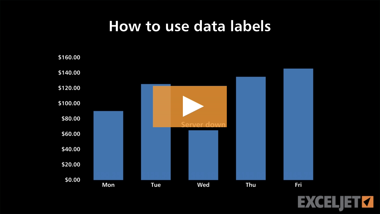
Excel tutorial: How to use data labels
Custom Chart Data Labels In Excel With Formulas - How To Excel At Excel Follow the steps below to create the custom data labels. Select the chart label you want to change. In the formula-bar hit = (equals), select the cell reference containing your chart label's data. In this case, the first label is in cell E2. Finally, repeat for all your chart laebls.

how to add data labels into Excel graphs — storytelling with data
How To Change Y-Axis Values in Excel (2 Methods) Right-click anywhere in the chart to open the drop-down menu of settings. Scroll to the option labeled "Select Data" and click on it. This opens the data dialog menu and allows you to change the settings and data of the chart's axes. 3. Click "Switch Row/Column" In the dialog box, locate the button in the center labeled "Switch Row/Column".
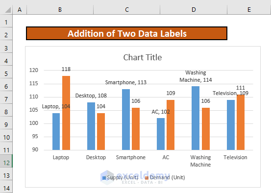
How to Add Two Data Labels in Excel Chart (with Easy Steps ...
How to Add a Marker Line in Excel Graph (3 Suitable Examples) - ExcelDemy Then select the whole data range B4:D18 and then go to Insert Tab > Charts group. From there, click on the Recommended Charts. After that, a new window will open. In that window, select the Clustered Column chart as shown in the image below. Click OK after this. You will see a new chart with both the Columns ( Revenue) and Line ( Column 1) present.

How to Add Axis Labels to a Chart in Excel | CustomGuide
support.microsoft.com › en-us › officeEdit titles or data labels in a chart - support.microsoft.com If your chart contains chart titles (ie. the name of the chart) or axis titles (the titles shown on the x, y or z axis of a chart) and data labels (which provide further detail on a particular data point on the chart), you can edit those titles and labels.
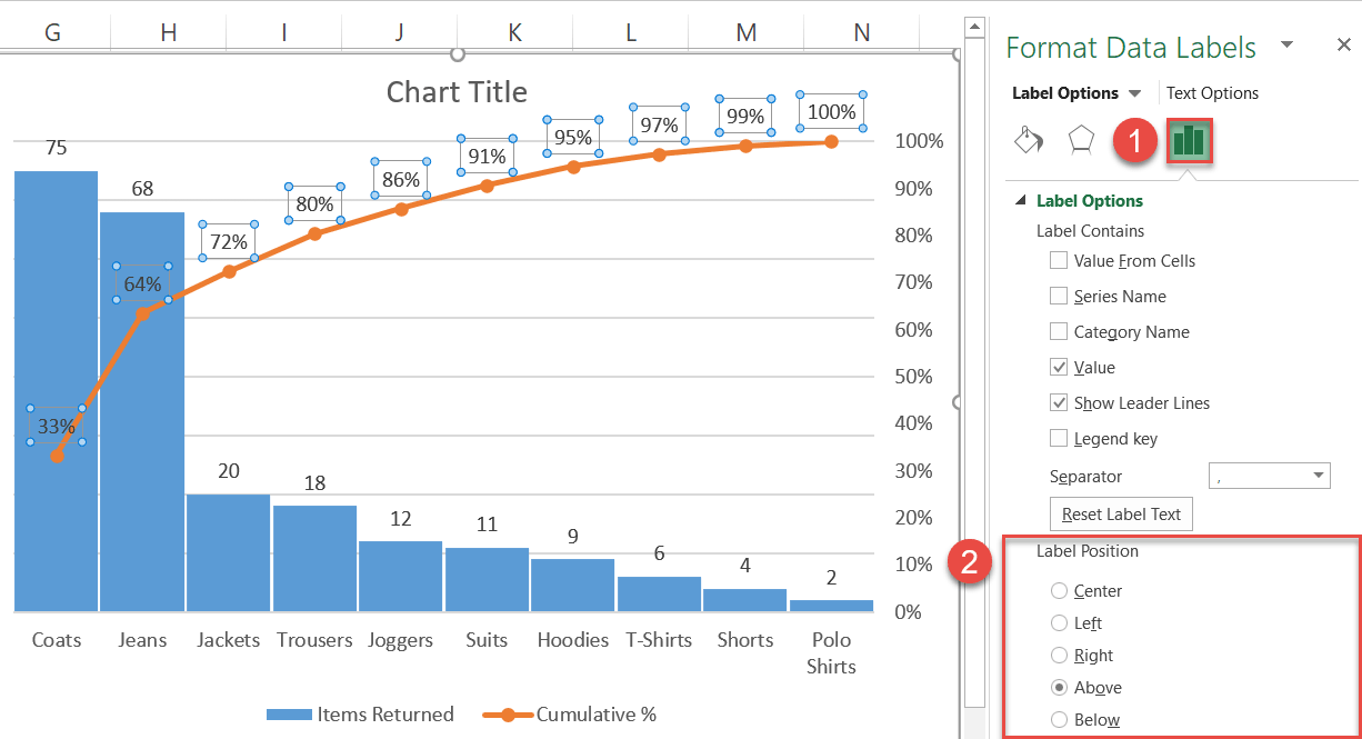
How to Create a Pareto Chart in Excel – Automate Excel
How To Add Data Labels In Excel - ksmu.info To get there, after adding your data labels, select the data label to format, and then click chart elements > data labels > more options. After picking the series, click the data point you want to label. Source: temotips.blogspot.com. Using excel chart element button to add axis labels. Click the chart to show the chart elements button.

How to insert data labels to a Pie chart in Excel 2013
Excel: How to Create a Bubble Chart with Labels - Statology Step 3: Add Labels. To add labels to the bubble chart, click anywhere on the chart and then click the green plus "+" sign in the top right corner. Then click the arrow next to Data Labels and then click More Options in the dropdown menu: In the panel that appears on the right side of the screen, check the box next to Value From Cells within ...

How to add total labels to stacked column chart in Excel?
support.microsoft.com › en-us › officeAdd or remove data labels in a chart - support.microsoft.com Depending on what you want to highlight on a chart, you can add labels to one series, all the series (the whole chart), or one data point. Add data labels. You can add data labels to show the data point values from the Excel sheet in the chart. This step applies to Word for Mac only: On the View menu, click Print Layout.

How to Add Two Data Labels in Excel Chart (with Easy Steps ...
Excel - adding new data points to an existing chart I am trying to add data points to an existing chart. The new data has been added to the table in the related spreadsheet. When I right-click on one of the three series shown in my chart and then choosing "select data" the Select Data Source window which appears states that "the data range is too complex to be displayed".

How to Add Two Data Labels in Excel Chart (with Easy Steps ...
Data Labels in Excel Pivot Chart (Detailed Analysis) Next open Format Data Labels by pressing the More options in the Data Labels. Then on the side panel, click on the Value From Cells. Next, in the dialog box, Select D5:D11, and click OK. Right after clicking OK, you will notice that there are percentage signs showing on top of the columns. 4. Changing Appearance of Pivot Chart Labels
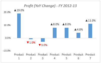
Color Negative Chart Data Labels in Red with downward arrow
› documents › excelHow to add data labels from different column in an Excel chart? This method will introduce a solution to add all data labels from a different column in an Excel chart at the same time. Please do as follows: 1. Right click the data series in the chart, and select Add Data Labels > Add Data Labels from the context menu to add data labels. 2.

Dynamically Label Excel Chart Series Lines • My Online ...

How to Add Total Data Labels to the Excel Stacked Bar Chart ...

microsoft excel - Adding data label only to the last value ...
Excel Data Labels: How to add totals as labels to a stacked ...

Adding rich data labels to charts in Excel 2013 | Microsoft ...

How to Show Percentage in Pie Chart in Excel? - GeeksforGeeks

Add Data Labels for Total to Stacked Columns in #Excel | wmfexcel

How-to Use Data Labels from a Range in an Excel Chart - Excel ...

Add or remove data labels in a chart

How to Place Labels Directly Through Your Line Graph in ...

Display Customized Data Labels on Charts & Graphs

Add or remove data labels in a chart

424 How to add data label to line chart in Excel 2016

How to add live total labels to graphs and charts in Excel ...
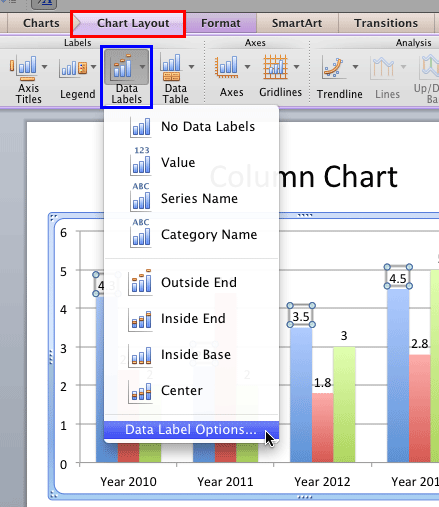
Format Data Label Options in PowerPoint 2011 for Mac

Microsoft Excel Tutorials: Add Data Labels to a Pie Chart

Add a Data Callout Label to Charts in Excel 2013 – Software ...

How to add or move data labels in Excel chart?
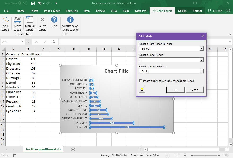
Add Labels to XY Chart Data Points in Excel with XY Chart Labeler

Adding Data Labels to Your Chart (Microsoft Excel)

Adding rich data labels to charts in Excel 2013 | Microsoft ...
/simplexct/BlogPic-idc97.png)
How to Create a Bar Chart With Labels Inside Bars in Excel
How do i add Data labels on the Pareto Line for the Pareto ...
Post a Comment for "42 how do you add data labels to a chart in excel"