45 excel data labels above bar
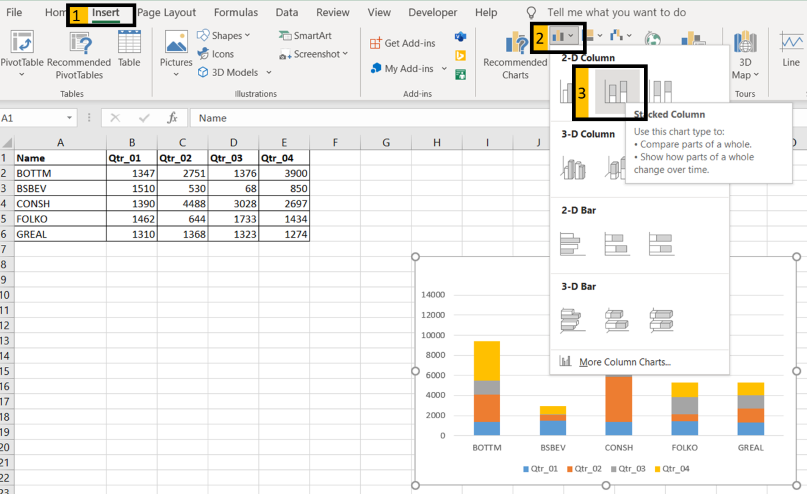
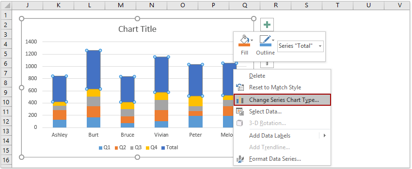
Showing percentages above bars on Excel column graph 0. The easy answer is you can edit the pivot table: -Right-click on the column showing series and goto pivot table options. -Click on Show values as an option. -Click on the percentage of grand total. -Enjoy :) Note: Although it will change the original values also to percentage. How to add total labels to stacked column chart in Excel? Add total labels to stacked column chart in Excel Supposing you have the following table data. 1. Firstly, you can create a stacked column chart by selecting the data that you want to create a chart, and clicking Insert > Column, under 2-D Column to choose the stacked column. See screenshots: And now a stacked column chart has been built. 2.
Add a DATA LABEL to ONE POINT on a chart in Excel To format the font, color and size of the label, now right-click on the label and select 'Font'. Note: in step 5. above, if you right-click on the label rather than the data point, the option is to 'Format data labelS' - i.e. plural. When you then start choosing options in the 'Format Data Label' pane, labels will be added to all ...
Excel data labels above bar
stacked column chart for two data sets - Excel - Stack Overflow Feb 01, 2018 · The output I want is to show years on the horizontal axis and having a country represented in a stacked column that piles up monthly data on the side of the column of the other country (like the chart made using Google Charts as explained in the the thread linked above. The solution should look that sample: How do you put values over a simple bar chart in Excel? 1) Select cells A2:B5 2) Select "Insert" 3) Select the desired "Column" type graph 4) Click on the graph to make sure it is selected, then select "Layout" 5) Select "Data Labels" ("Outside End" was selected below.) Custom data labels in a chart - Get Digital Help Select a single data label and enter a reference to a cell in the formula bar. You can also edit data labels, one by one, on the chart. With many data labels, the task becomes quickly boring and time-consuming. But wait, there is a third option using a duplicate series on a secondary axis. The animated image above shows you dynamic custom data ...
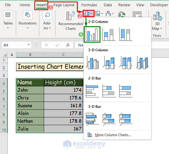
Excel data labels above bar. How to Make a Bar Chart in Microsoft Excel - How-To Geek To insert a bar chart in Microsoft Excel, open your Excel workbook and select your data. You can do this manually using your mouse, or you can select a cell in your range and press Ctrl+A to select the data automatically. Once your data is selected, click Insert > Insert Column or Bar Chart. Various column charts are available, but to insert a ... How to Add Total Data Labels to the Excel Stacked Bar Chart For stacked bar charts, Excel 2010 allows you to add data labels only to the individual components of the stacked bar chart. The basic chart function does not allow you to add a total data label that accounts for the sum of the individual components. Fortunately, creating these labels manually is a fairly simply process. Bar Chart in Excel (Examples) | How to Create Bar Chart in Excel? - EDUCBA Step 2: Go to insert and click on Bar chart and select the first chart. Step 3: once you click on the chart, it will insert the chart as shown in the below image. Step 4: Remove gridlines. Select the chart go to layout > gridlines > primary vertical gridlines > none. Step 5: select the bar, right-click on the bar, and select format data series. How-to Add Centered Labels Above an Excel Clustered Stacked Column ... Step-by-Step tutorial is available at: I posted how you can easily create a clustered stacked column chart in...
how to add data labels above Line and Stacked Column chart Stacked Column Chart - Since there is more than one value per column, hence there is no concept of above in this case. Just consider one column on top of another. Lower column has no concept of above. In this case, you have to manually move them above the lower and other top columns. But in case of Line chart, you should get all the options. How to Add Data Labels to an Excel 2010 Chart - dummies Use the following steps to add data labels to series in a chart: Click anywhere on the chart that you want to modify. On the Chart Tools Layout tab, click the Data Labels button in the Labels group. None: The default choice; it means you don't want to display data labels. Center to position the data labels in the middle of each data point. HOW TO CREATE A BAR CHART WITH LABELS INSIDE BARS IN EXCEL - simplexCT 8. In the Format Data Labels pane, under Label Options selected, set the Label Position to Inside End. 9. Next, in the chart, select the Series 2 Data Labels and then set the Label Position to Inside Base. 10. Then, under Label Contains, check the Category Name option and uncheck the Value and Show Leader Lines options. 11. How to Create a Bar Chart With Labels Above Bars in Excel In the Format Data Labels pane, under Label Options selected, set the Label Position to Inside End. 16. Next, while the labels are still selected, click on Text Options, and then click on the Textbox icon. 17. Uncheck the Wrap text in shape option and set all the Margins to zero. The chart should look like this: 18.
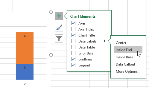
How-to Add Centered Labels Above an Excel Clustered ... The first thing we need to do is set up our data for the chart. The data setup for this Excel dashboard chart is as follows with the Clustered Stacked Column ... data labels outside of bar graph | MrExcel Message Board Select all contiguous cells Click here to reveal answer M murphm03 Banned user Joined Dec 14, 2012 Messages 144 Oct 30, 2013 #2 click on the bar you want to change-go to layout tab-data labels-outside end J johns99 Board Regular Joined Jun 11, 2013 Messages 212 Office Version 365 Platform Windows Oct 31, 2013 #3 Data Table in Excel (Types,Examples) | How to Create Data ... Data Table in Excel Example #1 – One-Variable Data Table. One-variable data tables are efficient in the case of analyzing the changes in the result of your formula when you change the values for a single input variable. Use case of One-Variable Data Table in Excel: Excel tutorial: How to use data labels If you have more than one data series, you can select a series first, then turn on data labels for that series only. You can even select a single bar, and show just one data label. In a bar or column chart, data labels will first appear outside the bar end. You'll also find options for center, inside end, and inside base.
How to add live total labels to graphs and charts in Excel ...
Excel, giving data labels to only the top/bottom X% values 1) Create a data set next to your original series column with only the values you want labels for (again, this can be formula driven to only select the top / bottom n values). See column D below. 2) Add this data series to the chart and show the data labels. 3) Set the line color to No Line, so that it does not appear! 4) Volia! See Below! Share
charts - Showing percentages above bars on Excel column graph ...
Data Labels above bar chart - Excel Help Forum Re: Data Labels above bar chart You can link the data labels to other cells to display anything you want. Free addin to link labels to cells Attached Files 1142048b.xlsx (21.0 KB, 18 views) Download Register To Reply Similar Threads Pie chart data labels By Duck1986 in forum Excel Charting & Pivots

How To Show Or Hide Data Labels On MS Excel? | My Windows Hub
How to Create Monte Carlo Models and Forecasts Using Excel ... To begin the Data Table, add a new sheet to your Monte Carlo workbook and name it Data. Then enter the labels, which are shown in bold in the preceding figure. The Seq (sequence) column is convenient for several reasons. To create the column… Enter the value 1 in cell B4.
Adding value labels on a Matplotlib Bar Chart - GeeksforGeeks
Add or remove data labels in a chart - support.microsoft.com Right-click the data series or data label to display more data for, and then click Format Data Labels. Click Label Options and under Label Contains, select the Values From Cells checkbox. When the Data Label Range dialog box appears, go back to the spreadsheet and select the range for which you want the cell values to display as data labels.
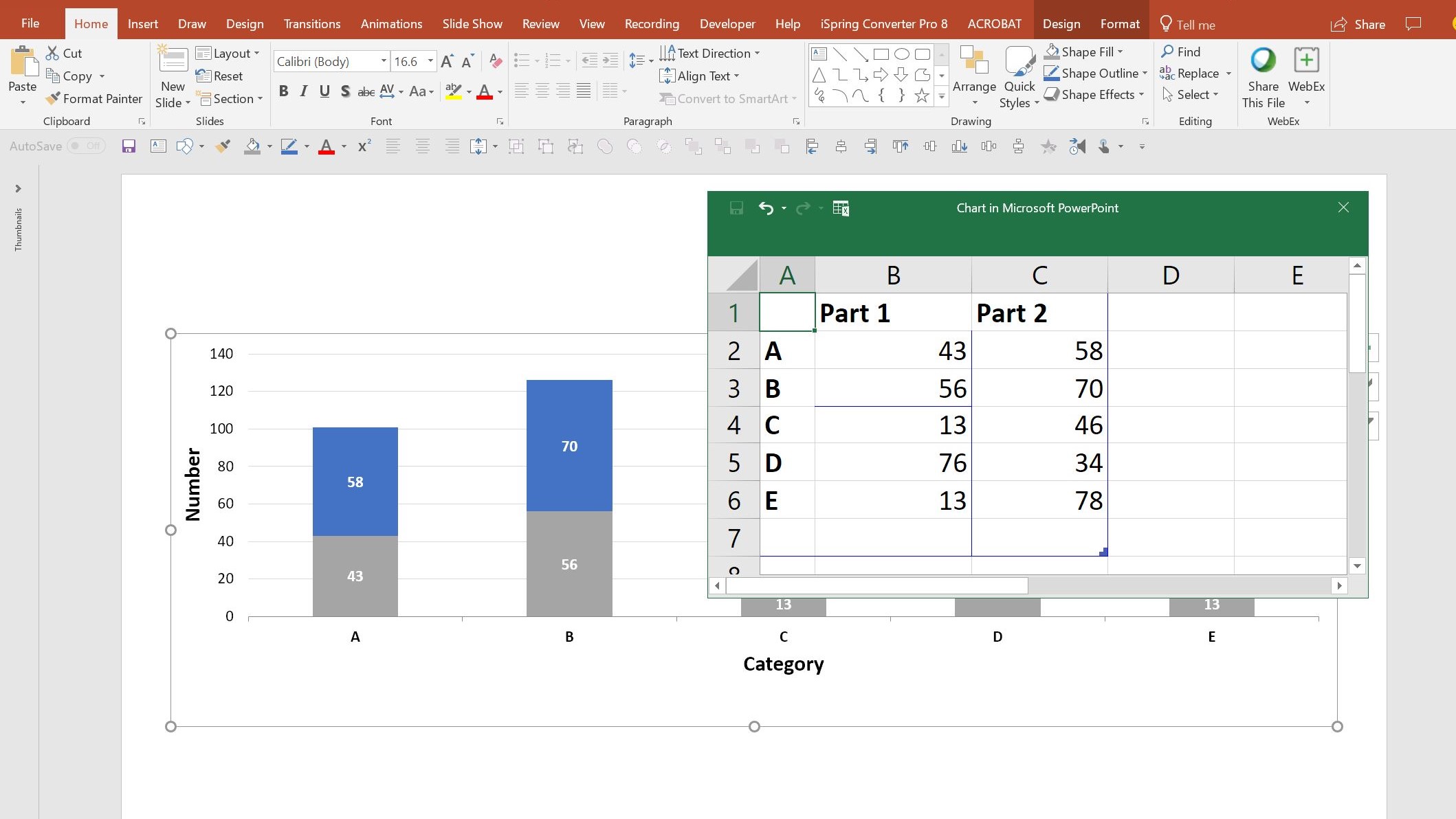
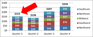
How to add total labels to stacked column chart in Excel?
How to Create Bar of Pie Chart in Excel? Step-by-Step Adding Data Labels. To be able to see the actual percentage of each portion/ category, adding data labels would be quite helpful. To add and format data labels to portions in your Bar of pie chart, follow the steps below: Click anywhere on the blank area of the chart. You will see three icons appear to the right side of the chart, as shown below:
How to Show Percentages in Stacked Column Chart in Excel ...
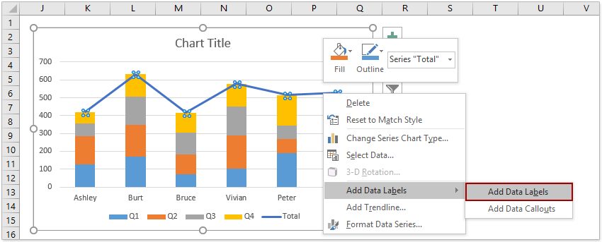
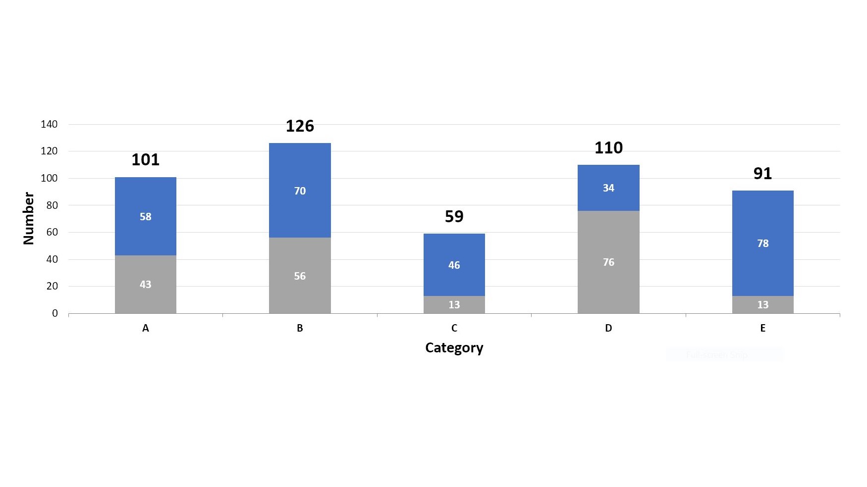
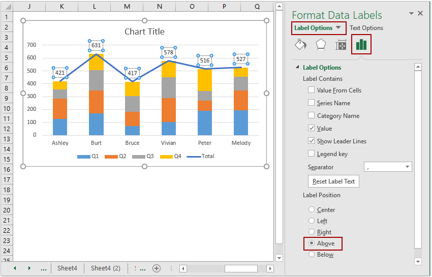
How to Add Total Values to Stacked Bar Chart in Excel Step 4: Add Total Values. Next, right click on the yellow line and click Add Data Labels. Next, double click on any of the labels. In the new panel that appears, check the button next to Above for the Label Position: Next, double click on the yellow line in the chart. In the new panel that appears, check the button next to No line:

Add Total Values for Stacked Column and Stacked Bar Charts in ...
Histogram with Actual Bin Labels Between Bars - Peltier Tech Select the chart, then use Home tab > Paste dropdown > Paste Special to add the copied data as a new series, with category labels in the first column. You don't see the new series, because it's a series of bars with zero height. But you should notice that the wide bars have been squeezed a bit to make room for the added series.
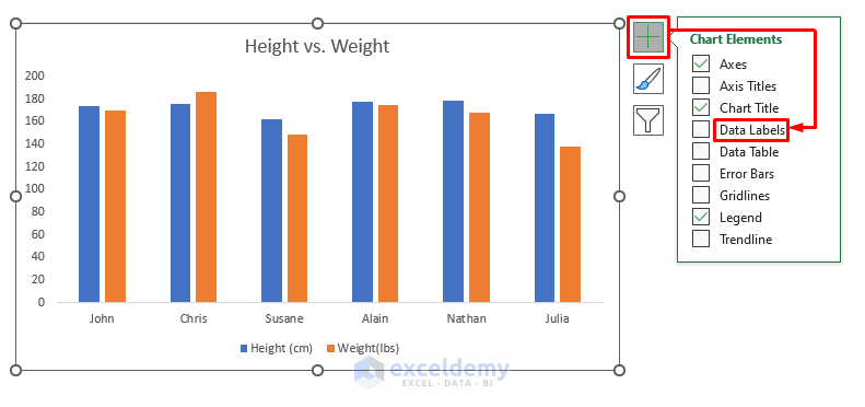
How to Add Data Labels in Excel (2 Handy Ways) - ExcelDemy
data labels not showing- options? - Power BI I have a bar chart and the data labels do not show on two of the three bars. It appears to be due to the bars being closer together, is there anyway to adjust the spacing or force the labels to appear above and or below? Solved! Go to Solution. Labels: Labels: Need Help; Message 1 of 7 11,424 Views 0 Reply. 1 ACCEPTED SOLUTION ...

Showing the Total Value in Stacked Column Chart in Power BI ...
Move data labels - support.microsoft.com Click any data label once to select all of them, or double-click a specific data label you want to move. Right-click the selection > Chart Elements > Data Labels arrow, and select the placement option you want. Different options are available for different chart types.
Format Data Label: Label Position - Microsoft Community
How to add or move data labels in Excel chart? - ExtendOffice 2. Then click the Chart Elements, and check Data Labels, then you can click the arrow to choose an option about the data labels in the sub menu. See screenshot: In Excel 2010 or 2007. 1. click on the chart to show the Layout tab in the Chart Tools group. See screenshot: 2. Then click Data Labels, and select one type of data labels as you need ...

Add Labels ON Your Bars
How to Create Address Labels from Excel on PC or Mac - wikiHow Mar 29, 2019 · Enter the first person’s details onto the next row. Each row must contain the information for one person. For example, if you’re adding Ellen Roth as the first person in your address list, and you’re using the example column names above, type Roth into the first cell under LastName (A2), Ellen into the cell under FirstName (B2), her title in B3, the first part of her address in B4, the ...

How to Show Labels Above Bar in a Horizontal Bar Chart
Prevent Overlapping Data Labels in Excel Charts - Peltier Tech Overlapping Data Labels. Data labels are terribly tedious to apply to slope charts, since these labels have to be positioned to the left of the first point and to the right of the last point of each series. This means the labels have to be tediously selected one by one, even to apply "standard" alignments.
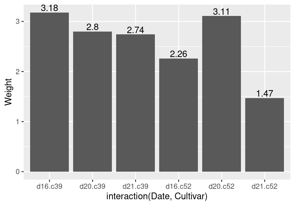
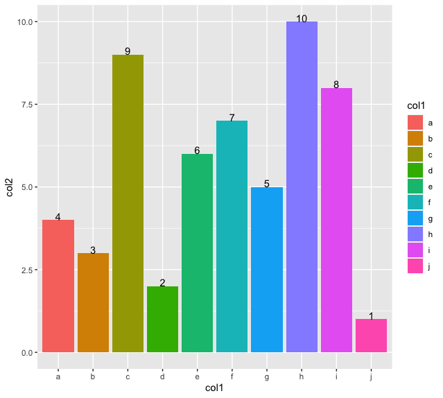
3.9 Adding Labels to a Bar Graph | R Graphics Cookbook, 2nd ...
Custom Excel Chart Label Positions • My Online Training Hub Custom Excel Chart Label Positions - Setup. The source data table has an extra column for the 'Label' which calculates the maximum of the Actual and Target: The formatting of the Label series is set to 'No fill' and 'No line' making it invisible in the chart, hence the name 'ghost series': The Label Series uses the 'Value ...
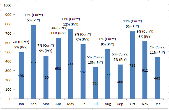
Add Multiple Percentages Above Column Chart or Stacked Column ...
How to Rename a Data Series in Microsoft Excel - How-To Geek Jul 27, 2020 · A data series in Microsoft Excel is a set of data, shown in a row or a column, which is presented using a graph or chart. To help analyze your data, you might prefer to rename your data series. Rather than renaming the individual column or row labels, you can rename a data series in Excel by editing the graph or chart.
/simplexct/images/Fig4-h1198.jpg)
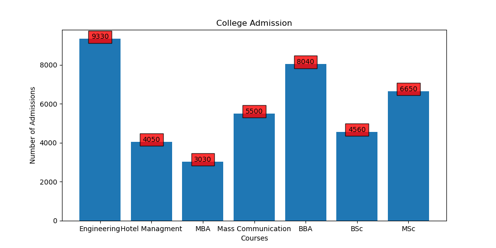
How to Create a Bar Chart With Labels Above Bars in Excel
Data labels on the outside end of error bars without overlapping? The easiest way to do this is to simply add 'data labels' and then replace the numeric value for the desired letter (instead of individually adding text boxes). Yet, one still has to manually move each data label/letter above the error bar because excel does not have this function.

Custom data labels in a chart
How to Change Excel Chart Data Labels to Custom Values? - Chandoo.org First add data labels to the chart (Layout Ribbon > Data Labels) Define the new data label values in a bunch of cells, like this: Now, click on any data label. This will select "all" data labels. Now click once again. At this point excel will select only one data label. Go to Formula bar, press = and point to the cell where the data label ...

how to add data labels into Excel graphs — storytelling with data
Excel Charts - Chart Elements - tutorialspoint.com Step 4 − Click the icon to see the options available for data labels. Step 5 − Point on each of the options to see how the data labels will be located on your chart. For example, point to data callout. The data labels are placed outside the pie slices in a callout. Data Table. Data Tables can be displayed in line, area, column, and bar ...
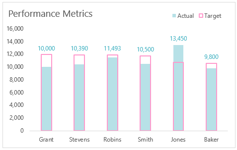
Custom Excel Chart Label Positions • My Online Training Hub
Data Bars in Excel (Examples) | How to Add Data Bars in Excel? - EDUCBA There are two kinds of Data Bars available in Excel. Select Gradient if you present both bar and numbers together or if you are showing only bars select Solid. You can change the color of the bar under Manage Rule and change the color there.
How to Add Data Labels in Excel (2 Handy Ways) - ExcelDemy
Custom data labels in a chart - Get Digital Help Select a single data label and enter a reference to a cell in the formula bar. You can also edit data labels, one by one, on the chart. With many data labels, the task becomes quickly boring and time-consuming. But wait, there is a third option using a duplicate series on a secondary axis. The animated image above shows you dynamic custom data ...

Change the format of data labels in a chart
How do you put values over a simple bar chart in Excel? 1) Select cells A2:B5 2) Select "Insert" 3) Select the desired "Column" type graph 4) Click on the graph to make sure it is selected, then select "Layout" 5) Select "Data Labels" ("Outside End" was selected below.)

Add Total Values for Stacked Column and Stacked Bar Charts in ...
stacked column chart for two data sets - Excel - Stack Overflow Feb 01, 2018 · The output I want is to show years on the horizontal axis and having a country represented in a stacked column that piles up monthly data on the side of the column of the other country (like the chart made using Google Charts as explained in the the thread linked above. The solution should look that sample:

Format Data Labels in Excel- Instructions - TeachUcomp, Inc.

Combination Clustered and Stacked Column Chart in Excel ...

Add or remove data labels in a chart

Adding rich data labels to charts in Excel 2013 | Microsoft ...
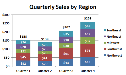
How to Add Totals to Stacked Charts for Readability - Excel ...
/simplexct/images/Fig7-vfc0a.jpg)
How to Create a Bar Chart With Labels Above Bars in Excel

Excel Chart Label - Adding, removing, positioning chart labels
How to add total labels to stacked column chart in Excel?

Apply Custom Data Labels to Charted Points - Peltier Tech

Display Customized Data Labels on Charts & Graphs

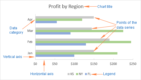
Excel charts: add title, customize chart axis, legend and ...
Move and Align Chart Titles, Labels, Legends with the Arrow ...
How-to Add Centered Labels Above an Excel Clustered Stacked ...

Custom Excel Chart Label Positions • My Online Training Hub

Adding rich data labels to charts in Excel 2013 | Microsoft ...
How to add percentage or count labels above percentage bar ...

How to Customize Your Excel Pivot Chart Data Labels - dummies
How to add live total labels to graphs and charts in Excel ...
How to Add Totals to Stacked Charts for Readability - Excel ...

How to add or move data labels in Excel chart?
How to add total labels to stacked column chart in Excel?
Chart with a Dual Category Axis - Peltier Tech
How to make a bar graph in Excel

How can I hide 0% value in data labels in an Excel Bar Chart ...
Post a Comment for "45 excel data labels above bar"